An Experimental Contribution on the Origin of Mass
To date, apart from non-verifiable hypotheses, there is no theory available to unite electromagnetism, quantum theory and gravitation with each other. The experiment presented below shows a way out of this crisis of physics. In this experiment it will be proved, that mass has to be associated with the self-induction energy of moving charges. The proof was performed with a highly sensitive balance. The experimental setup is shown in figure 1:
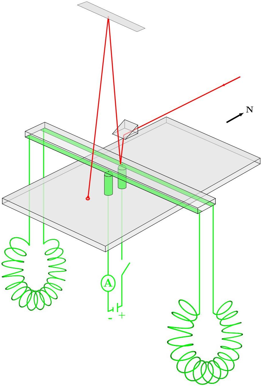
The balance beam is made of glass and coated on the lower surface with two aluminum stripes of equal width and length. The coating procedure is performed in one coating charge, in order to avoid differences between the aluminum stripes and to provide identical conduction paths. The beam center is positioned on two equal steel balls contacting the aluminum layer that provide the current supply from the DC source (shown below). At each end of the balance beam a respective toroid is conductively connected to the aluminum stripes. The two toroids are identical with their sense of the helix being opposed to each other: The right-hand and the left-hand toroid correspond to a screw with right-hand thread and left-hand thread resp. A laser beam (red) was used as a light pointer, because a very small effect was anticipated. This laser beam is reflected by one of the aluminum layers in the center of the balance beam and indicates very sensitively the deflection of the balance beam.
To avoid conceivable magnetic interference, the balance was positioned with the Earth’s magnetic field parallel to the toroids.
After the current had been switched on, a remarkable deflection of the balance beam was observed, i.e. while the weight of the right-hand threaded toroid decreased, the weight of the left-hand threaded toroid increased.
Reversing the polarity provided the same deflection of the balance beam, i.e. again the weight of the right-hand threaded toroid decreased, the weight of its counterpart increased.
Removing and reversing the complete arrangement (balance beam and toroids) from left to right, i.e. the right-hand threaded toroid now was on the left side and its counterpart on the right side, after applying the current the deflection of the balance was found to have reversed too. This means, again the weight of the right-hand threaded toroid decreased and the weight of its counterpart on the other side increased - also independent from the current polarity.
Accordingly, the mass changes as a function of helicity have also been transferred to the other side resp.
For verification of the experiment the following measurement conditions are given:
- Balance beam:
- - Float glass, both sides blank, 500 mm x 20 mm x 2mm
- - Aluminum coating: 2 stripes, width 8 mm each, thickness 2 µm
- - Uncoated clearance: 4 mm
- - Diameter of the steel support balls of the beam: 3.9 mm;
- Toroids:
- - Core material of each toroidal coil: foamed polystyrene, non-conducting
- - Size of the foamed polystyrene rings:
- * inner ring diameter: 95 mm, outer ring diameter 145 mm
- * Diameter of the polystyrene body: 50 mm (145 - 95);
- - Weight of a polystyrene toroid: 4.3 g;
- - Number of wire turns on each toroid: 135;
- - Diameter of the coil wire: 0.6 mm;
- - Material of the coil wire: aluminum
- - Total weight of the wire of one toroid: 85.6 g;
- Laser:
- - He-Ne laser at a wavelength of = 633 nm
- - Optical path of the light pointer: 4.8 m;
- Power:
- - 400 mA DC;
- Calibration:
- - the scale of the balance was calibrated by means of 1‑mg weights;
- Results:
- - At a current of 400 mA, one side of the beam became lighter by at least 0.1 mg and the opposing side became heavier by at least 0.1 mg.
Summary:
- Moving charges generate mass by self-induction.
- The energy thus produced is determined by the geometry of the path of these charges and therefore bound to the location of the movement, i.e. virtually stored. This fixed energy must be associated with the mass.
- Not only groups of moving charges, but also single charges must generate mass by self-induction, because by their movement they interact with their own field.
- This self-induction of single charges opens up the door to the comprehension of the quantum theory.
The presented experiment was inspired by: B. Heddisch, Betrachtungen zum Thema Atom »
Die vorliegenden
"reflections on the atom"
wurden am 04. Oktober 1972 abgeschlossen und vom Verfasser unterzeichnet.
Für den Inhalt ist ausschließlich der Verfasser verantwortlich.
![]()
Albert Einstein‘s famous words
"God does not roll dice!"
have inspired this paper.
After some probing steps and false starts, incredibly convincing explanations have incidentally been found for the Pauli principle, the magneto-mechanical anomaly (spin), the Heisenberg uncertainty principle, the wave-particle-duality the light as well as for the problem of the universal physical constant.
Encouraged by these reference points, it has been found that Planck’s constant (quantum of action) cannot be a universal physical constant but instead describes of the reflexive cause-effect-complex of a charge. In other words, a charge can interact with itself in the atom by interacting with its own electromagnetic field.
By means of this postulate we succeeded in calculating the value of Planck’s constant within close approximation.
By progressing along these lines, some self-interaction mechanisms will be designed that represent elementary particles, such as protons, neutrons etc., and which describe the nuclear forces in terms of coupled self-interaction energies. Thereby it will be shown that the mass/-energy equivalent E=m0c2 is generated by such self-interaction effects.
In the concluding “Fantastic Outlook” we will see that interesting and new perspectives in understanding nature can be opened up.
Since the introduction of the Bohr postulates, quantum theory has interpreted a large number of natural phenomena correctly and, most important, has described them perfectly in mathematical terms.
Today, this advanced domain of physical science has expanded so much that a single individual could hardly be successful in getting even an almost complete overview of all fields of knowledge covered by quantum theory. Often years of education are necessary before a physicist becomes an expert in one of the great many specialized fields.
Considering the speed of development of quantum theory, we have to acknowledge that the era of tremendous and rapid progress seems to be over since every new finding is likely to be gained with a great deal of experimental and computational effort, and that discussions about new hypotheses seem to absorb more and more time.
Similarly, one also gets the impression that in the light of various experimental results, quantum theory will be faced with problems that are difficult (or even impossible) to solve.
Maybe quantum theory really has reached a limit that no longer allows considerable progress in the recognition of nature?
If this is true, one can expect that the basic principles of this huge theoretical structure are not solid enough designed to support said structure and that one possibly has to start again from the very beginning.
This paper pursues such a goal. It intends to doubt the correctness of the foundations of quantum theory, since it is exactly these foundations that include apparent contradictions for the layperson almost without exception. These include the dualism of light (which could also be assigned a wave packet that should actually dissolve immediately). Also included is the electron spin that should be so immense that even the highest speed admitted by the relativity theory – the speed of light – is surpassed many times over. Moreover, quantum theory also comprises the famous uncertainty principle that forbids any penetration beyond a specific limit, etc.
While these “contradictions” are not considered contradictions by the expert since quantum theory is based on the idea that there is no causality of single natural processes, within the limits of that theory there exists only a causality of probabilities and on this basis it can even be shown that there isn’t any illustrative and, thus, causal model of the atom as yet.
Maybe it is just this opinion that deserves critical re-evalutation, since actually each classical description is based on the causality principle; and this principle, often confirmed by experience, also makes use of quantum theory as far as possible.
Now let us just assume someone would claim that this principle applies to all natural processes. Immediately, each expert could disprove such an assertion using ample evidence.
Let us further assume that nature actually behaves causally in all its details, that even all evidence opposing such an opinion is correct and that only the standpoint on which this evidence is based requires revision – then a strange contradiction evolves: First, the expert’s path toward further development of this theory is blocked due to the above-mentioned numerous evidence. Secondly, while the layperson would be able to take a causal viewpoint he could not cope with the expert’s arguments because he lacks knowledge about quantum theory and cannot understand the expert’s counterarguments adequately. On the other hand, the layperson is obliged (in the interest of science) to hold his view despite all inadequacy of proof.
For this reason the author claims the right to take a causal viewpoint without proving it beyond all doubt. Therefore, the reader should regard the following heuristic considerations as merely an opinion and a (perhaps interesting) adventure, forgiving the arbitrariness that is necessary for such a position.
Der Weg
At the beginning of this consideration a question should be asked that refers to the critical comments of the introduction. It is known that the emission of an electromagnetic wave of a Hertz’ oscillator can be described very well and illustratively. However, this idea will fail immediately if you try to develop a clear descriptive model of the emission of a light quantum from an atom. This is one of the peculiarities of quantum theory. On the other hand we cannot see any significant difference if we compare the products of the two emission mechanisms (i.e., the electromagnetic waves) and therefore have every right to ask: Why in one of two methods to create a physical object the mechanism should be clear while not in the other one? This question is only a means to approach the field of quantum theory from another perspective (rather than the common one). We will therefore follow such a path allowing us to develop a causal image of nature and begin with the equations that describe the emission mechanism of an atom.
It is to be assumed that the handling of our subject does not imply the desire to explain each character or symbol precisely since such explanations generally disturb one’s train of thoughts. Instead, we will only try to use those characters which can be found in any textbook of physics, and, if necessary, introduce clearly understood characters.
Now we will have a look at the following equations:
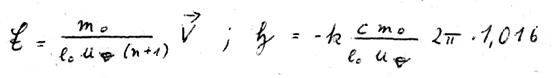
(energy of a light quantum)
(equation of the speed of light)
and
III
(difference in energy levels of two electrons „orbiting” around a nucleus)
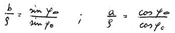
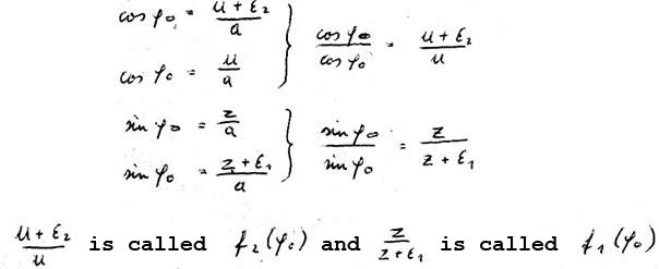
Eliminating  and extending by
  (Fig. 1):
IV
or:
V
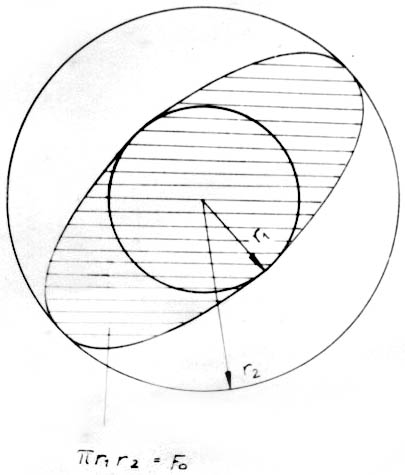
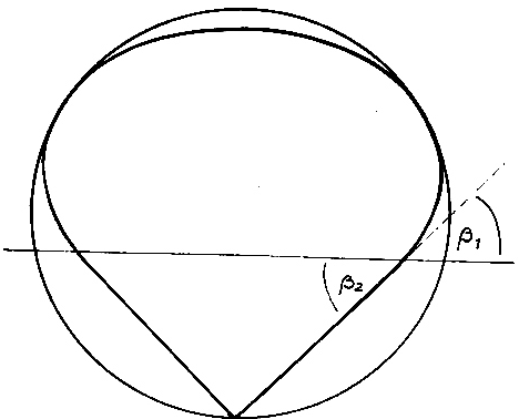
Essentially, the Sommerfeld fine structure constant is seen in the framed term on the right side of the equation; now the left side of the equation becomes quite interesting. Here we find the relation between two geometric quantities, multiplied by the wavelength of the emitted (or absorbed) light. Maybe the curve encircling the elliptic area is the orbit on which the electron travels while the light quantum is emitted?
There is much in favour of this assumption. First, the fact that the difference between two radii (a level difference) is part of the numerator on the left. We consider the level difference as the difference of two electrical quantities. Secondly, the denominator contains an area that each physicist will relate to a magnetic field. Certainly, one may feel tempted to get to the bottom of the emission mechanism if one imagines that the electron oscillates between the two (emission-free) orbits on the elliptic curve until its energy difference is consumed and it swings into one of the two orbits. When “jumping up” or “jumping down” it should emit an electrical field and - when it reaches the highest possible speed (when touching the inner orbit) - a magnetic field.
However, this was not actually the object of our considerations; we want to gain another perspective by applying minor conversions. We use the following equations:
VI
Hence:
VII
This conversion is aimed at clearing the Sommerfeld fine structure constant of c because then, as is well known, we obtain the speed of the electron on the innermost orbit of the hydrogen atom. This provides better understanding and clarity in our equation. Thus, in the denominator one finds the speed of the electron on the lowest orbit of the hydrogen atom.
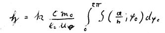
Considering equation VII carefully and using our imagination, we may ask, that if equation VII is the equation of the emission, what does the equation of a steady orbit look like? Here we integrate over a closed area. Perhaps for a steady orbit we have to integrate over an annular surface? We will attempt it since such an experiment will not cost more than a failure. Actually, how often a wrong calculation has resulted in a reasonable idea! Consequently, we will replace the denominator by such an integral over a ring surface (Fig. 2):
VIII
is replaced by the diameter of the electron ( eØ ) has to be used.
So the denominator of the left side of the equation becomes:
IX
a rotational speed within a steady orbit. This is amazing!
Now, let's insert z = 1 (VII) into the equation and compare the two denominators. We obtain:
X
on the innermost orbit of the hydrogen atom!
Now we come to the decisive question, since everything that has been written down until now has been used to elaborate the following statements. To sum up (under the condition that our speculations so far are basically true): if the atomic nucleus is within the area to be integrated, light will be emitted (or absorbed). However, if the nucleus is not located within this area, we will have a steady orbit. Hence, why not always integrate over the nucleus?
Since we have identified the area as the abovementioned magnetic field, we now claim:
The magnetic field that should be generated by an electron during its movement within a stationary orbit (meeting the quantum condition), is simply zero at the nucleus, i.e. there isn't any magnetic field. If, though, the magnetic field does not exist at the nucleus, then such an electron cannot radiate on its orbit, and must therefore remain on a stable orbit. This is because an electrical field and a magnetic field are required, when a light quantum is emitted. Thus, maybe the electron moves around the nucleus on an orbit, that simply does not generate a magnetic field at the nucleus. But because the nucleus fixes the electron on a circular or elliptic orbit due to the Coulomb attraction, it is not possible for the moment, to allow for the selection of orbits other than circles or ellipses.
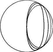
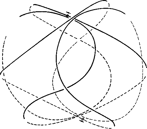
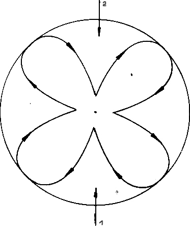
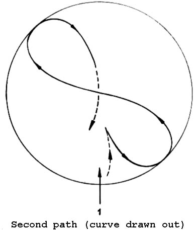
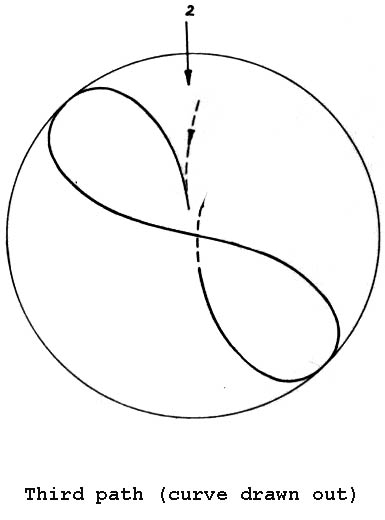
On the other hand, for the simplest case of the hydrogen atom's innermost orbit quantum theory calculates a spherically symmetrical charge distribution. For this reason (or better: reference point) let us allow the whole spherical surface, whose radius should be equal to that of the circular orbit, to be used in the selection of suitable orbital paths. Thus, we restrict ourselves to the simplest case, i.e. to the orbit of the electron on the innermost orbit of the hydrogen atom. We hereby let the electron travel at constant speed - required by quantum theory for this orbit - while allowing the electron to be laterally deflected and initially not taking care about why the electron can be expelled from an even (circular) orbit. A hollow glass ball is best suited for demonstration. The orbit shown in Fig. 3 is meant to be a suggestion for such an orbit. Four small circular paths are orbiting the spherical area such that they continuously merge into each other.
At this point we will perform the first arbitrary act. Namely, we demand the angular-momentum conservation law to be no longer applicable to this orbit. While still allowing the numerical value of the angular momentum to be constant we demand that the direction of the angular momentum vector be no longer a constant. Thereby we are completely inconsistent with quantum theory. What's more: it is just the constancy of the angular momentum (caused by the strict regulation of Planck's constant) that provides the basis of all theories on elementary particles. This point implies one of the main contradictions of quantum theory: it requires constancy of the angular momentum and calculates a spherically symmetrical charge distribution! This point can be called a crossroad. Either we decide for the angular momentum and get a non-causal world or we decide for the spherically symmetrical charge distribution and attempt to build a causal world. We decide to take the second way, and in this regard do not consider this step of changing over to such an orbit as an arbitrary act.
Viewing this orbit from the center of the sphere, i.e. from the nucleus, four curved drop-shaped subareas can be seen; whereby each of these orbited subareas could generate a magnetic field at the nucleus.

If, however, one accepts the following hypothesis, then actually no magnetic field can be generated at the nucleus:
But as none of the four subareas is continuous in terms of the spatial derivative of the path (from the view of the nucleus) there would be actually "magnetic calm" at the nucleus. Besides, this "calm" exists in the entire interior of the sphere. This assertion (hereinafter referred to as "magnetic field theorem") is really not very extreme if one bears in mind that the magnetic field is an eddy current field.
An eddy, however, should only arise, if the generator " the charge " follows a continuous and, in terms of the derivative, closed continuous curvature; otherwise, the generation of an eddy in a frictionless environment is unimaginable. Also, this theorem is not contradictory to macroscopic experience. Therefore, we surmise that the greatest uncertainties in quantum theory lie in the interpretation of magnetic effects.
Initially, we provide the radius of the 4 small circular paths. So let's have a look at Figure 4.
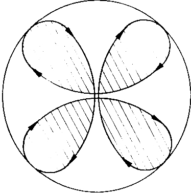
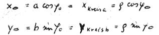
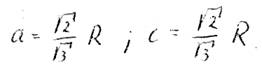
(Note: the reader is well-advised to have a hollow glass ball at hand in order to trace this orbit. He will make the following explanations transparent in the true sense of the word.) First, we look in the direction e - f (Fig. 5). The path takes the shape of a rosette whose four lobes each consist of the branch of an ellipse. We accept only one ellipse, and from the myriad of ellipses passing through the origin of coordinates and touching the enveloping circle, we calculate the ellipse that has a common point with the circle and the straight line x = y (Fig. 6). The semi-axis of this ellipse equals the radius of the small circular paths of our orbital path:
IX
R = radius of the sphere
The fact, that this path (seen from direction e - f) and its spatial derivative as well are continuous, needs no detailed explanation, since it was calculated under this condition. To prove the absence of kinks over the entire surface of the sphere, we have to look at this curve from two other directions as well, and check the continuity of the derivative. It will be sufficient if it is proven for the direction a - b. If the continuity of the derivative can be shown here, then it will be identical with the third independent view (eg. b - c). It can easily be shown that  (Fig. 7).
Therefore, we have a completely continuous and kink-free closed path before us that circumscribes an octahedron that fits into the sphere. Further, we will have achieved the spherically symmetrical charge distribution required by quantum theory if we conduct the electron (initially by force) along this orbit. This orbit is even by pieces.
Now, we cheerfully tackle the answer to the question of how the electron shall be caused to wobble. In any case, there must be a force that does not perform any work (i.e. no changes in speed); only changes in direction should be permitted. This must be - as we assume - the Lorentz' force and we will look around for magnetic fields. They are also there; we only have to look in the direction of the arrows 1, 2, 3, or 4 and we will see continuous and in terms of their spatial derivative closed continuous ellipses that do not contradict our magnetic field theorem formulated at the beginning. Should the electron really swim on its own magnetic fields without the nucleus becoming aware of (Fig. 8)?
This will be the explanation for the standing De Broglie waves that had to serve as a model for the idea of steady orbits so far. Thus, these "standing waves" would turn out to be rotating magnetic fields.
This idea of rotating magnetic fields is the first successful application of our model based on the real relationships set up by nature. We assess them to be an indication of the accuracy of the model and will be looking meanwhile for other indications (before we try to answer the question about the cause of the electron's wobbling characteristics). We will use this method of thinking ahead just to check if the specified orbital model offers even more related signs, which would provide a clear, unrestrained picture of natural processes and, whether a further consideration makes sense at all. Thus, we raise the following question: How many electron orbits of this kind can we allow on such a spherical shell if the atomic number is correspondingly increased? We have assumed the electron to swim on its own magnetic field. Therefore, we must state now: only one second electron fits onto the spherical shell (Fig. 9). This second electron must be located opposite the first on each point of the orbit (it shall be hidden behind the nucleus in such a manner that the two electrons do not "see" each other). Every further electron that is added would terminate this nice game of hide-and-seek, and according to the magnetic field theorem, "notice" the magnetic fields of the other two electrons. The harmony would come to an end and the stationary orbit would be corrupted.
This is a illustrative interpretation of the Pauli exclusion principle. In spite of this, we still have to make up for something. We still owe a clear interpretation of the electron spin since without a spin we cannot explain the Pauli principle. After all, it is known that the introduced spin puts the electron into such a powerful rotation that it collides with the theory of relativity. However, the orbit introduced by us copes with lower speeds. Again we look toward the direction e - f and see a magnetic field generated by 4 orbiting lobes which is not in contradiction to our magnetic field theorem (Fig. 10). This is the spin.
Due to our theory of a hide-and-seek game for two electrons, this rosette surface is orbited by the two electrons in the opposite direction and we will obtain the correct result for the anti-parallel orientation of the spin magnets for the inert gas helium in its ground state.
Nevertheless, we are obliged to calculate the gyro-magnetic ratio of the Einstein-de-Haas experiment for our spin model to show that this model also corresponds here to the actually given values:
XII
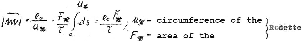
The magnetic moment is (in terms of the average of the period of a single revolution):
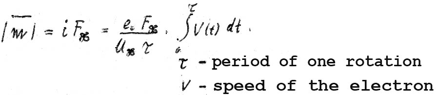
We obtain:
XIII
The angular momentum (also in terms of the average of the period of rotation) is:
XIV

Based on this, we can claim that the integral  equals
  .
.
One can prove this in two different ways, e.g. by considering the fact that the (mean) angular momentum is composed of two rotations: one forward rotation within each quadrant and one backward rotation when changing from one quadrant into another. We provide this proof by means of a very illustrative auxiliary orbit. This orbit may be substituted by three single orbits whose mean angular momentum can immediately be read from the orbital curve so that we can do without complicated mathematical equations. For the first part of this orbit see Fig. 11.
Thus, we allow the electron to orbit at exactly the speed that it had at an equivalent point on the original orbit; we just do not allow it to dive through the center of the rosette, but stop it here promptly to send it to the next quadrant at the same speed (for clarity’s sake the orbits have not been drawn up to the center).
We have made an error in the second and fourth quadrants and will correct it immediately by means of the second and third orbits. This is done by cutting open the first orbit at points 1 and 2 and inserting the second and third orbits in between them (Figures 12 u. Figures 13):
All these manipulations are permissible because the orbital changes are performed at a point of time, when the contribution to the angular momentum integral is zero.
Hence, the mean angular momentum of the first orbit must be  . It is obvious that for the other two orbits the mean angular momentum is 0. However, for the complete coverage of our construction consisting of three auxiliary orbits, we need twice the time necessary for the given rosette orbit.
Thus, for our auxiliary orbit, we have obviously got the mean angular momentum of an orbit that has actually been travelled twice. The immediate consequence is:
XV
Hence, only half the area can contribute to the area speed for such a “forward angular momentum with reverse gear” (Fig. 14).
From XIII and XV now follows the gyromagnetic ratio of the “spin”:
XVI
Now we may claim for our model: there is no electron spin in terms of quantum theory.
Clarity can now also be seen in the question of why there is a direction quantization in the Stern-Gerlach experiment. This is simply because the electrons do not like to be disturbed in their finely woven magnetic field spin. Just as they reject admitting a third partner in a spherical shell, they also reject disturbances of their rhythm by external fields. This is best achieved by turning their axis e - f toward the external field. Then all 4 magnetic fields are indistinguishable and no one is priviledged. Still another argument speaks against the existence of the electron spin in terms of quantum theory: it is not known that free electrons – e.g. cathode rays or electrons that are generated by the ß-decay of radioactivity – show a Stern-Gerlach effect. On the other hand, it does not make sense to fight against an idea which does not actually claim to be illustrative; the spin of the electron should only be a substitute model for processes that cannot be specified in detail. Likewise, except for its mathematically correct formulation, the atomic model of quantum theory does not claim to be illustrative, so that in a discussion about the drawbacks of the previous model it’s like preaching to the choir since this model simply does not exist.
Let’s return to the question we have not yet answered. It was speculated that the Lorentz’ force can be responsible for the electron wobbling on its orbit. Therefore, we carefully conduct the electron along the four small circular paths. Afterwards, we attempt to calculate one of the four magnetic fields (e.g. direction 1) and then calculate the Lorentz’ force by formulating  . Subsequently, this Lorentz’ force should be equated with the centrifugal force acting on the small circular paths. Now it becomes exciting:
Having succeeded in obtaining such an equation we could think about how to calculate Planck’s constant. Due to the equivalence of the centrifugal force and the Coulomb attraction of the nucleus, there is a second equation that fixes the electron to the spherical shell and contains h– due to the “quantization rule” -!
It remains to be seen if we will have immediate success with this procedure. In any case, we have serious doubts about whether or not the quantity h is a universal physical constant. Even for the following reasons the existence of h as a universal physical constant is very uncertain: all natural processes can be described by means of a measurement system that can do with 3 independent dimensions. Therefore, it must be possible to describe all physical laws by means of a measurement system that is based upon three universal physical constants. However, we have four so-called universal physical constants. Consequently, one of them must be redundant:
One does not tend to easily doubt the first three quantities, but rather the fourth one, particularly since it demonstrates in the form of the fine structure constant that it is not independent of e0, and c.
In a word, let us attempt the calculation of  by means of the Biot-Savart law, although we know for sure that this is a wrong approach and that we will certainly fail any time. Nevertheless, the risk must be taken since we hope to find such arguments that may be helpful.
XVII
As we have established our magnetic field theorem, we will be looking for only in the spatial direction that corresponds to the projection of the ellipse shown in Figure 8. (For clarity, the drawing is made such that the viewer sees the ellipse at a slight incline.)
But for a current filament remaining in a given plane, the Biot-Savart law can slightly be simplified (Fig. 15).
XVIII
XIX
This means to calculate exactly on the circumference of the ellipse, which is certainly wrong. Nevertheless, let's take the risk:
XX
We simplify the equation because  on the ellipse is difficult to specify (Fig. 16).
XXI
This equation is valid because  and
and  are the result of tilting a circle that is travelled at constant speed.
Hence:
XXII
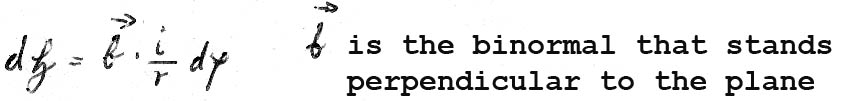
So we have reached the point at which the calculation cannot be continued because  equals
In the same way, the binormal gives us a hard time because it stands vertically to our plane of projection and not - as needed - on the second small circular path that is tilted against the plane of projection (equation XXI does not affect the direction of the binormal). Nevertheless, we continue our calculation using false values - just to learn from our mistakes. Certainly, there is an unknown principle hidden behind this n the content of which will possibly be revealed in part due to the errors in our calculation.
Next, we forcefully rotate the binormal toward the desired direction and call the indefinable integral: 
Hence:
XXIII

Now we equate the Lorentz' force with the centrifugal force on the small circular paths:
XXIV
XXV
So, and now we give free rein to our imagination:
We assume that  contains ambiguous solutions and that it is a linear function of
 because then a quantum rule would be established:
XXVI
This would mean that  could apply! If we calculate the numerical value of
 , we will see that it is only about 3 powers of ten away from the value of Planck's constant. Nevertheless all of these speculations are only built on sand; now let's eliminate the errors and learn from the defeat.
We have reached the point to formulate the decisive theorem:
The Biot-Savart law is useful for calculating a magnetic field from any current-flow in a conductor loop. But how do we find its strength, direction etc.? For sure we will find it by measuring the effect of this magnetic field on any other magnet or at least a charge e0 But as we know that molecular magnets do not exist, the use the Biot-Savart law requires at least two electrons: one electron that generates the field and a second whose changes are still to be determined. Thus, the Biot-Savart law describes the dependencies of at least two electrons to each other (as practically all laws of physics are designed to examine cause and effect on different objects).
How, though, will things look, if cause and effect occur on one single object? Certainly it can't be excluded that an electron might eventually interfere with its own magnetic field (which should be the case for our atomic model). In other words, do we really want to deny the existence of the magnetic field for this specific case?
That is simply impossible, since by experience we all know the classical term of self-induction. This physical effect, applicable to the movement of a group of electrons following the magnetic field theorem, should also apply to a single particle. This conclusion can immediately be derived by using the fact that in a group of electrons a single electron cannot be distinguished from the other ones. Therefore, let us consider one single electron of this group. It generates (like all the other electrons) the magnetic field. And as is well known, the partial magnetic field generated by this single electron affects all the other electrons. But because the electrons are indistinguishable from each other, the "partial magnetic field" must also react to its generator, quod erat demonstrandum
Now let's extend still another theorem that we have just mentioned. What will happen, if cause and effect occur on one electron and have to be controlled? Of course a control is no longer possible because any intervening operation upon this mechanism would inevitably lead to changes. This is the real content of the Heisenberg uncertainty principle, namely that Planck's quantum of action provides an "intervention limit".
Therefore, we can deduce that:
- the application of the Biot-Savart law must fail because it was based on false assumptions,
- the unknown principle to be discovered can only be as follows:
That is why it is first an action (effect) and secondly a quantum and why quantum laws cannot be measured but rather have to be guessed!
Incidentally, exactly for this reason the application of the formula of the Lorentz' force fails. From now on, it is necessary in any case to precisely check all mathematical formulations and physical conceptions for their applicability.
First, we want to introduce the terms "self-interaction" and "external interaction", of course in accordance with of the above formulated theorem.
Further, we will look for starting points for a mathematical treatment of the task. First, this is rather discouraging since all quantum effects are of probabilistic nature, albeit, in full harmony with our concept. This is because each physical interaction mechanism can develop in two directions: the particle either interacts with itself or it interacts with other particles. And here we have the origin of the dualism of matter: In case of external interaction we have classical physics; in the case of self-interaction - quantum physics. But if we interpret everything in classical terms (the external interaction), then an uncertainty principle will establish itself as an insurmountable barrier that is precisely determined by the value of the interaction constant of self-interaction of a charge.
If we consider the successful interpretations achieved by the model so far from the aspect of self- or external interaction, they are now seen in a much better, brighter light. Now the game of hide-and-seek of the Pauli principle, for example, can only be interpreted such that, due to this orbital arrangement, the self-interaction remains undisturbed. In the same way, we can now understand the "deflection" found in the Stern-Gerlach effect.
Nevertheless, we are getting sidetracked from our task - the calculation of Planck's constant. We are looking for a quantum effect that enables us to find mathematical laws of self-interaction. As we do not want to get a mixture of classical and quantum physics that can provide only half the truth (the other half relates beyond doubt to the part of classical physics that is uninteresting to us), we are looking for a quantum effect that occurs with certainty, not just with probability. Moreover, said quantum effect must be characterized by a total absence of friction - for how should a particle rub itself? And thirdly, as a consequence of the missing friction, we demandthe law of conservation of energy to apply to this process. Consequently, we are looking for a modest perpetuum mobile that remains in an endless motion, though without producing or consuming energy.
This, of course, is superconduction. Then let us use the supplementary equations of the Maxwell equations, found phenomenologically by v. Laue and London that are satisfied by the supercurrent, and interpret them as follows: in the case of the superconduction, an external magnetic field produces antiparallel orientation in the directions 1, 2, 3, or 4 of our model. This hypothesis, however, requires a more detailed explanation.
As is well known, there are various kinds of magnetism of matter. We - in accordance with quantum theory - interpret ferromagnetism as a spin magnetism oriented toward the external magnetic field - of course in the sense of the introduced "orbital spin". This magnetism is definitely that part of our orbit's magnetic field which acts outwardly. Therefore, it corresponds to the external interaction and, thus, shows classical behavior, while orienting with respect to the external fields and appearing as paramagnetism - provided there are no grid alignment rules . The diamagnetism, however, must be attributed to the self-interaction. Due to our statements provided for the direction quantization and the Pauli principle, we have to realize that self-interaction - as long as it "does not want to be destroyed" - always tries to avoid the external fields or, if impossible, build up a counter field. However, since the superconductor is ideally diamagnetic and, moreover, meets our requirements of missing friction, it should be expected that the equations satisfied by the supercurrent are really the equations that control self-interaction. However, now we have to demand the absence of any external interaction for the electrons generating the supercurrent, i.e. the spin moments of said electrons are saturated pairwise. This requirement consistent with the explanation of superconduction provided by quantum theory is also considered to be an indication for the validity of our model. Further we see that for the spin saturation of our model - namely for full occupation of the spherical shell - the two electrons have actually the same sense of rotation around one of the given spatial directions (e.g., direction 1). This means that for spin saturation (no external interaction) the fields of self-interaction will not offset each other; i.e. diamagnetism may indeed exist.
Thus, we will interpret the two supplementary equations found by London and v. Laue as self-interaction equations and will explain very roughly the path to be followed: It should only be mentioned that the unproductive way we have taken thus far must not be followed again. According to the theorems previously formulated, it makes no sense to speak about Lorentz' force and centrifugal force as usually.
This is why we have to adopt a totally different approach that satisfies the conditions set up before. So, using the two equations for
 and
and  mentioned above, we will try to apply the law of conservation of energy - that should still be valid - and calculate h.
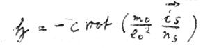
The attentive reader will certainly have realized that the above calculations were inconsistent with respect to the applicable measurement system . Now, we decide to use the Gaussian CGS system, first writing down the two equations for
and :
XXVII
XXVIII
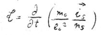
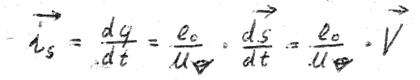
where  is the supercurrent and ns the concentration of the electrons involved in superconduction. First, we face the task of rewriting the two equations for one electron. In doing so, for the term we will proceed as usual:
XXVIX
Thus, we view at our path - as agreed upon - for example from direction 1 and select - for the path taken by the electron - the entire path the electron draws on a projection perpendicular to direction 1 during one revolution. We designate this term as  . Now let's turn to the term ns:
| ns = | number of electrons involved in the superconduction | = | n |
| second | sec. |
We also rewrite the second (we do not make too serious an error if we accept only integral numbers of revolution):
1 second ≈ number of the revolution periods * revolution period
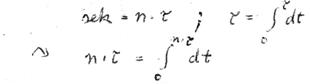
XXX
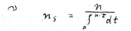
Now, since we do not want to sum up many electrons, we will use another concept that enables us to express ns for one electron. For this purpose we provide the following example: If each of 6 electrons performs one revolution per second, the following equation will apply:
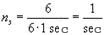 .
.
The result will be the same if one electron is made to orbit six times faster:
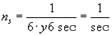
This is what we have achieved: we consider the number n as a number of revolutions that can be performed by one electron in a defined period and now require this number to be an integer. We justify this requirement by our magnetic field theorem that forbids the discussion about the existence of a magnetic field at all unless at least one complete revolution has been performed. Thus, we have illustratively introduced the main quantum number n.
Thus, we write:
Consequently, this equation should apply also for magnetic fields.
The same procedure applies to the term ns in the equation of the electric field; but to explain this we have to go into greater detail:
As we demanded at the very beginning, there should be "magnetic calm" at the nucleus when maintaining our model orbit. From this we had derived this orbit to be nonradiative, since for energy output (radiation of light quanta) both an electric field and a magnetic field are required. We now conclude in the same way: if there is a magnetic field only for one complete revolution, then for a definite energy value the electric field will only exist, if exists. This means that only integral numbers n will qualify for the electric field as well because we want to apply the law of conservation of energy. Therefore, we generalize:
This important theorem pricks up our ears since we actually know such energy packets in the form of light quanta. This means that the light quanta (the electromagnetic waves) are such products of self-interaction. Hence, the dispute about the assignment of wave packets, which can be assigned to the particles in terms of de Broglie waves, amounts to nothing: in the same way as light quanta are products of their self-interaction, also particles (initially the charged ones) show self-interaction - provided that only combinations of
and
are admissible - meaning that they are waves in nature. In other words, they are able to interact with themselves.
But now let's return to our quantum number to be selected for the field. After all, we must not select it equal to n magn., because we have required self-interaction to occur only if the electron has already terminated one revolution, i.e. that a magnetic field already exists. Hence:
Hence, we can write for the equations XXVII and XXVIII::
XXXI
XXXII
But we are not satisfied even with these equations since there are functions of time ( ) in front of the integrals. While this notation may certainly be correct for the summation over many electrons (with superconduction), it is wrong for one single electron. Therefore, we must require that - if the particle is to interact with itself - all terms dependent on t be part of the integrals. Thereby with the -field, the differentiation
 and the integration over t offset each other because V on the ellipse only depends on t; i.e. the partial differential and the total differential as a function of time are identical. This notation is not arbitrary since certainly is a function of the location in the superconductive material if we consider many electrons. (It is known that the interior of the supercrystal is shielded by a "supercurrent" flowing on its surface.)
Therefore, we examine an electron on the crystal surface:
XXXIII
XXXIV
If we look at these two equations and keep in mind that the product of and
must appear when calculating the energy - that we actually want to provide at some point of our calculation - then the term n (n + 1) would appear in the denominator of this product!
This may be the reason why the term  must stand for the square of the angular momentum in quantum theory! Actually, we have provided an illustrative interpretation earlier: self-interaction is only possible if one revolution has already been performed (due to the magnetic field theorem). We assess this numbers game again as an indication of the validity of our approach and now start calculating the magnetic field according to equation XXXIII. We notice with satisfaction that, unlike the Biot-Savart law, this magnetic field is not branded by the disadvantage of the impossibility of the expected results.
Yet another small correction is necessary in this equation, and as usual we explain it by using the magnetic field theorem: in the following, we will not adopt τ as the total time needed by the electron to follow its "wobble trajectory" but only as the revolution period for the ellipse visible in direction 1 since there is no magnetic field beyond this continuous and in the spatial derivative continuous space curve! The same holds truefor calculating
only for this ellipse while not considering the other parts of the trajectory.
Therefore, we write:
XXXV
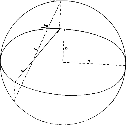
 in Cartesian coordinates (Fig. 17)
Hence:

a radius of the small circular path: ![]()
b obobtained by a simple geometric relationship from the parameters of the octahedron: ![]()
Now we write in cylindrical coordinates by introducing the following terms (Fig. 18):
We prefer these terms, because they greatly facilitate integration:
and
We obtain: 
Since we like to express all terms using circle parameters (which - as mentioned above - considerably facilitates integration), we introduce the following terms (Fig. 19):
Hence:
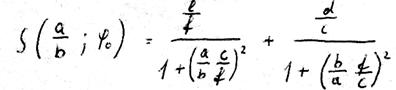
The right-hand expression within the bracket we call S . This function S is continuous over
  and has no discontinuity points with reference to its derivative. This function can no longer be expressed by simple means. However, it can very easily be generated graphically by drawing the ellipse and its circumscribed circle and measuring the distances indicated in Fig. 20.
XXXVI
For our case with the quantities a and b it is a function that slightly differs from 1 and describes a sinusoidal curve.
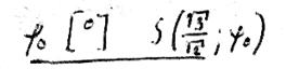 | |
| 0 | 1,0 |
| 10 | 1,0024 |
| 20 | 1,0065 |
| 30 | 1,097 |
| 40 | 1,0130 |
| 50 | 1,0270 |
| 60 | 1,0130 |
| 70 | 1,0085 |
| 80 | 1,004 |
| 90 | 1,0 |
Now, this function can very easily be graphically integrated and we obtain:
XXXVII
For we obtain:
Now all terms have been reduced to the circle and we can calculate ![]() :
:
XXXVIII
Initially, we just want to notice two interesting results: First, the field ![]() appears without quantum number because this is cancelled after integration.
appears without quantum number because this is cancelled after integration.
Further, apart from ![]() , there remain only constants in the equation. This is the mathematical formulation of our magnetic field theorem. In any revolution, one electron can generate only one magnetic field the strength of which mainly depends only on the trajectory travelled by the electron. Thereby only that part of the trajectory that encloses a continuous and in the spatial derivative closed continuous space curve.
, there remain only constants in the equation. This is the mathematical formulation of our magnetic field theorem. In any revolution, one electron can generate only one magnetic field the strength of which mainly depends only on the trajectory travelled by the electron. Thereby only that part of the trajectory that encloses a continuous and in the spatial derivative closed continuous space curve.
![]() may contribute to the generation of the
may contribute to the generation of the
![]() field.
field.
Thus, we only have quantum rules because there is no continuous spectrum of elementary charges. Consequently, the root of all quantum rules lies in the fact that we find only one specific elementary charge in nature.
![]() field depends on the value of the ratio
field depends on the value of the ratio
![]() (actually contained in the S-function). If we now imagine - aside from our special example - any other ellipse with a much higher main axes ratio
(actually contained in the S-function). If we now imagine - aside from our special example - any other ellipse with a much higher main axes ratio
![]() we will see that the magnetic field has increased. This would mean that the greater the inclination of the travelled circular trajectory the larger the magnetic field in case of self-interaction, if it is examined under various inclination angles. For now, weleave this result, which definitely is inconsistent with classical experience, to revert to it later.
we will see that the magnetic field has increased. This would mean that the greater the inclination of the travelled circular trajectory the larger the magnetic field in case of self-interaction, if it is examined under various inclination angles. For now, weleave this result, which definitely is inconsistent with classical experience, to revert to it later.
Now let us start to calculate the energy of the particle. For this purpuse, we use the equations for
and
As mentioned above, to specify an energy value only makes sense if there is a magnetic field
, i.e. if the magnetic field theorem is satisfied, we must express
in such that only the component of
that can be recognized in direction 1 will be included into the calculation. That means that
 must be replaced by
 in the equation for

Now,
and
definitely stand vertically on top of each other and the difficulties once caused by the binormal are almost eliminated. But we have still to explain the „almost”:
has a negative sign. This fact would inevitably provide the absurd solution of a negative energy when calculating the product of
and
.
But in our attempts to explain the direction quantization of diamagnetism and superconduction, we have already found, that self-interaction - as far as it does not want to be eliminated - either avoids exterior fields or, if impossible, builds up a counter field. But as we have taken our
equation from superconduction, where exterior fields are measured, for the self-interaction we may now reverse the sign of
for the self-interaction:
XXXIX
Again, we add :
XL
There is one drawback in the two equations. This drawback has already been discussed with the
field for the function
 .
In case of the
field, the disadvantage is caused by the following situation: we have decided to calculate the self-interaction energy of a particle that shall ultimately be calculated from a product of
and
.
This self-interaction energy has to be a constant because we have found that one particle can interact with itself only if it has the size of one interaction energy quantum. This quantum should somehow be related with Planck's constant, so that h can be calculated. Now we come to the abovementioned disadvantage of
:
.
In case of the
field, the disadvantage is caused by the following situation: we have decided to calculate the self-interaction energy of a particle that shall ultimately be calculated from a product of
and
.
This self-interaction energy has to be a constant because we have found that one particle can interact with itself only if it has the size of one interaction energy quantum. This quantum should somehow be related with Planck's constant, so that h can be calculated. Now we come to the abovementioned disadvantage of
:
is not a constant because
is variable. In other words, no interaction energy quantum can be obtained for the energy. This contradiction - like the contradiction inherent to the
field - resolves very easily if we consequently apply the statements made above: in self-interaction there is no pure magnetic energy and no pure electrical energy as well.
But these two contradictions result from the classical idea of
and
and we still have no right to make a disparaging judgment unless we have calculated this self-interaction energy. Therefore, we consider
and
as slightly deformed copies of an image of nature that we can just perceive as blurred. This is because the means
(,),
tthat we use for observation simply do not allow us to see more sharply. Only the combination of
and
t? the self-interaction energy - will enable us to see more sharply since it exists within the range of self-interaction.
We expressly reiterate this idea because it is absolutely fascinating. Within the range of self-interaction, there exists only the product of
and
ei.e. an energy; hence it is useless to discuss all other kinds of energy such as pure electrical or pure magnetic energy since the two do not exist. That's why quantum theory may provide statements about energies, energy levels, energy quanta, energy jumps etc. We mention this again because we understand this statement - that can finally be traced back to our magnetic field theorem formulated in the beginning - as an important indication for our concept.
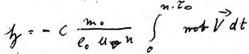
To calculate the self-interaction energy we use the equation that leads to the derivation of the Poynting vector for light quanta. We expect that this equation can readily be applied to the problem to be solved because, according to our concept, light quanta are products of self-interaction.
XLI
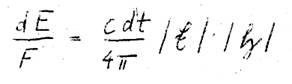
The differential of the energy flowing through the area F (that is perpendicular to the propagation direction of the light wave) is equal to the length, divided by 4π, of the parallelepiped that is perpendicular to the area F, multiplied by the absolute values of
and
that lie in the plane of the area F. Here the length of the parallelepiped is given by the path of the light beam with the speed c that has been traveled within the period of time dt.
Of course, we have to rewrite this equation - that (like the equations of superconduction) is of summary nature - for our electron, namely for one particle. To that end, arbitrary acts are necessary againand, hopefully, success will justify the unallowable means.
First, we replace the speed of light in the propagation direction of the wave by the speed of the particle in direction 1. We call this component Vz. Now, we look toward b-d and draw only that part of the orbit that is necessary to generate a closed ellipse visible in direction 1 (Fig. 21):
Hence, for Vz:
This equation is an approximation of Vz. Strictly speaking, again this should be an elliptical function which, though, does not deviate considerably from the proposed approximation.
Next, for the equation of the Poynting vector we write:
XLII
And after the integration over  from 0 to 2π (due to the magnetic field theorem):
XLIII
We now have the energy that would flow through the area F if only this ellipse were continuously travelled. This, however, is not true because in our model there are definitely points of time at which we do not find any energy in direction 1. This is the case when the electron travels those parts of the orbit that should not provide a contribution of energy.
This amount of energy given in equation XLIII only exists for one eighth of the complete revolution of the electron around the nucleus. And this eighth is only an approximation, as well. When calculating more precisely, we should change the integration limits in equation XLII continuously and then average the result. Since in our model this error can only be insignificant (all ellipses are not strongly "elliptic") we are satisfied with this one eighth.
However, for the Poynting vector exactly the energy is calculated that flows through the area F per unit time (e.g. per second). Therefore, we have to divide the right side of the equation by 8 too:
Now we come to use
und
and, for sake of clarity, write the equations XXXIX and XL as follows:
Anyway, the two quantities have some minor drawbacks. First, we will discuss the drawback of
suggested above:
is not a constant but for our case we demand E = const! This is because we, according to our expectations about a self-interaction quantum, have to set E = const since we want the law of conservation of energy to be valid also within the range of self-interaction. Secondly, we have to set E = const, if we want to take the modest perpetuum mobile of superconduction into account.
Therefore, we write our proven integral form for area F (that we of course identify with the area of the ellipse in direction 1) and proceed in the same way with these two quantities like we did before with ns:

(Fig. 22)
But as V0 is a variable of
, it must be put - for the self-interaction of a particle - under the integral. Hereby the difficulty of the variability of V0 and, thus, of E has been overcom:
XLIV
Now, as usual, we express the elliptical functions by the quantities of the circles:
XLV

Now
T , like
S
, is not an elementarily integratable elliptic function.
, like
S
, is not an elementarily integratable elliptic function.
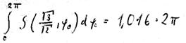
But it can be easily integrated graphically, too. In our case of the quantities a and b the integral takes on the value 0.50077 * 2π
It is thus a variable differing slightly from π.
Hence:
Now, let’s proceed to the aforementioned minor draw-back of
:
There is no component of
within the plane of the area F but
is perpendicular to this area. However, the Poynting vector is valid for energy fluxes for which
and
have a component within the plane of the area F. So, we first take note of this characteristic feature of the “particle wave” and continue calculating with the available component of
Otherwise, we would be forced to declare the magnetic field theorem wrong – and it was precisely this theorem that brought us a series of nice indications for the validity of our approach.
On the other hand, we do not see any reason why we have to expect absolutely the same rules for a charged particle as for photons because we still know too little about the mechanisms that cannot be strictly derived and, as we mentioned at the start, certain arbitrary acts cannot be avoided with our procedure.
Therefore, we write:
Now it becomes most interesting:
As we have discovered four such self-interaction mechanisms in the form of the four marked directions 1, 2, 3, 4 according to Fig. 4, E is consequently a quarter of the self interaction energy that an electron can generate on its complete wobbling orbit. Hence
From this follows:
XLVI
const. = E total = 4 ⋅ E =
We demand, as announced repeatedly, that E total = const. Moreover,
 has the dimension R2. This means that this equation contains Bohr’s angular momentum quantization rule:
XLVII
const. = E total = 4 ⋅ E =
This is due to the fact that there are only constants on the right side of the formula (apart from the marginal variability of m ≈ m0) nur noch Konstanten.
And now we turn our attention to the constant:
As superconduction appears in the direct vicinity of zero absolute, we may state: the electrons responsible for superconduction already adopt the lowest level of energy that an electron can adopt shortly before they reach zero absolute: they are already “frozen” shortly before the zero point. They have lost any kind of external interaction (as we have already demanded by the pair-wise spin saturation). Thus, their total self-interaction energy is the only energy they have. Consequently, this self-interaction energy must be equivalent to the lowest possible energy level of an electron, i.e. the rest energy
XLVIII
const. = m0c2
m being set to m = m0 we obtain with close approximation,:
XLIX
m0V0R=
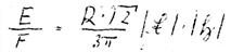
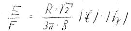
The constant within the dashed line should amount to the numerical value of Planck’s constant, which will be verified as follows:
For comparison, the experimental value of h is:
This result corresponds to the quantum of action given by nature except for a slight difference of approx. three per cent. We attribute the obtained deviation to the approximations. For the time being, the aim is reached by this result even though many questions concerning the causal view of the elementary processes remain to be answered. But we note that this coincidence with the natural constant h is not accidental, since the procedure demonstrated above, despite the arbitrary acts, does not lack a certain logic.
Apart from a few exceptions, we have collected indications so far that should confirm the validity of our considerations. And we consider the calculation of Planck’s constant as a first piece of evidence for the validity of our hypothesis. Planck’s constant is not a universal constant if a case can be found for which it can be calculated. Thereby, it is clear why all quantum theories only provide partially correct results: all of them believe this quantum to be a universal constant and so have to compensate all the difficulties inherent to this assumption for a lack of clarity, non-determinacy and artificial models such as spin, dualism etc. Consequently, Planck’s constant as a universal constant is the linchpin of all the theories about elementary particles. This outcome is
of tremendous importance and at first one does not know where to begin. Perhaps it will be best to start with an illustrative concept about the mechanism of self-interaction. Therefore, we let the electron travel along an orbit that satisfies the magnetic field theorem conditions in any spatial direction. Thereby, the orbit will perpetually intersect field lines. However, in this case the orbit itself must be a field line and field lines would permanently intersect each other. But we know that in nature intersecting field lines must not exist. For this reason, a part of the field lines are always pushed to the convex side of the orbit; for a closed continuous curve we obtain a spatial vortex if the electron terminates its orbit. This vortex is the magnetic field.
Now we know that apart from the guessed orbit of the electron, there are still other orbits that are known as ellipses until now. According to our concept, these orbits embody wobbling curves on rotational ellipsoids as shown in Fig. 23. On such rotational ellipsoids the four small circular paths are distorted into ellipses, the octahedron is stretched and the four spatial directions in which self-interaction can be observed, have straightened up. Furthermore, again we identify the spin rosette in direction e-f. Likewise on this orbit the product m* V * R = const., if we place the nucleus into one focus of the ellipsoid. At the same time, as in the spherical-symmetrical model, there is “magnetic calm” at the nucleus. We thus observe in the simplest case an electron that is revolving the hydrogen nucleus on such an orbit and we want to show that the ratio of the two ellipsoid axes satisfies the rules of both the magnetic and the secondary quantum number required by quantum theory. Only if this is successful, it will have been shown that h is really a constant on all possible orbits around the nucleus. Consequently, we have to prove that such an elliptical orbit will generate the Planck’s constant only if the elliptical integrals in our self-interaction equation contain the correct semi-axes values.
Anyway, we are optimistic because it is known that the elliptical functions are double-periodic
functions so that the possibility to “discover” even more quantum numbers in addition to the already introduced principal quantum number definitely does not seem to be hopeless – no, on the contrary, it must even be expected. Indeed, from the double periodicity inevitably follows that not two new secondary quantum numbers independent of each other can be found but only one; the other one must inevitably satisfy a simple ratio of a principal and an independent secondary quantum number. Of course, we assess this “strange coincidence” as an indication in terms of our hypothesis. But soon after writing down the determination equation for the semi-axes ratio this optimism is considerably dampened.
This would mean solving an equation as a determination equation for the semi-axes, which already becomes totally confusing when writing it down. Even the formulation of the functions in such an equation is so complex and leads to elliptical integrals with very complicated integrands that an elementary solution is no longer imaginable, particularly, if one keeps in mind the tools required (which of course are not available to the author). Thus, this proof must be postponed. (In the final comments we will revert to this problem.).
Now we turn our attention to the principles of atomic structure and ask if our model also here provides clear results in accordance with nature. Therefore, we imagine – according to the already known procedure – a naked nucleus that catches electrons one after the other. We do not have to discuss hydrogen and helium because we have found by explanation of the Pauli principle that these two cases are in accordance with the real conditions. The question about lithium is much more interesting.
Initially we observe that the two electrons travelling on the 1s orbit do not realize the 2s valence electron revolving outside because they are always inside the spherical shell generated by the 2s orbit and, thus, within the range of “magnetic calm”. Now we ask: Doesn’t the 2s electron “take notice” of the 1s electron? Here two options are possible: first we will discuss the possibility that the 2s electron can interact with the spin rosette in direction e-f.
This type of interaction, though, is impossible because the two 1s electrons simultaneously terminate one revolution and, thus, their respective magnetic fields offset each other. The second possibility would be the situation that the 2s electron “notices” and somehow “couples” the self-interaction of a 1s electron, e.g. in direction 1 (see Fig. 4), with its own self-interaction. This would be true if the period of revolution of the 1s and 2s electrons were identical due to the magnetic field theorem. As this is not the case, “disturbances” do not occur here. But let’s stick to the idea that the self-interaction of one electron could be “coupled” with the self-interaction of another electron. This would be the case if the two electrons would not belong to the same nucleus. As we have to demand both electrons to have the same revolution period, i.e. the two electrons have to coincide with respect to their principal (and certainly also secondary) quantum numbers, this could possibly be the explanation for a pure homopolar compound, e.g. for a
H2 molecule?. But as we know from quantum theory, this requires an anti-parallel spin-setting as a precondition. Indeed, we have to be prepared for this, as well, because the
H2 molecule has reduced its contribution to the external interaction in the case of two anti-parallel spin rosettes , i.e. the
H2 molecule is more similar to an inert gas than the single atom. Hence, the electron “prefers” the “undisturbed” self-interaction or the “slightly disturbed” or coupled self-interaction to the external interaction. How does such a “coupling” look like if the spin rosettes are anti-parallel to each other? The same will happen that has previously been discussed for superconduction: both electrons revolve in the same sense of revolution around direction 1! Thus, for the coupled self-interaction we obtain a result that is contrary to Lenz’s induction law: coupled self-interaction will generate a force of attraction only if the sense of revolution and the revolution period around the space direction , in which the coupling exists, are identical for the two partners. We should have to expect this result because otherwise the self-interaction could not exist under these conditions. And this is just the same result as provided by quantum theory: If the spins of the partners are arranged parallel to each other, a repulsive force will be generated. So, we can write down the following theorem:
Using the same arguments we can explain the ionic bond: a place exchange is done in favor of the “slightly disturbed” self-interaction. However, we have just strayed from the subject a bit and will return to lithium. We can add further electrons, knowing that each sphere and each ellipsoid shall be occupied by two electrons until the next one will be built up. It may happen, though, that very excentric orbits sometimes break out of the range of “magnetic calm” and “notice” the external s electron that is not protected against external interaction (Fig. 24). Consequently, we have to demand that these orbits must not be occupied before the orbit of the s type (spherical type) is completely occupied in order to be protected against external interaction.
This rule of thumb fails with chromium first, then for copper and finally will be violated more and more starting from niobium. This is due to the fact that we cannot explain the multi-particle problem using such a simple rule any longer – we cannot even overlook it. Thus, we can summarize by saying that our interpretation of the structure principle is also an indication for the validity of the path explained up to this point. And here the author would like to add some comments: the reader will certainly have noticed by the large number of quotation marks that a certain individuality is ascribed to the electron in the state of self-interaction. This kind of description should be interpreted as follows: we purposefully search for a universal extremal principle that contains the two self-interaction mechanisms (internal and external) and that allows to describe all natural processes as consistently as possible. To this end we have collected material and selected this kind of description. To provide such a principle, it is necessary to answer the following question: Which motive or reason is the crucial factor for the electron to “decide” for one type of interaction or the other? Only due to this we are still unable to explain dynamic processes occurring in the atom (e.g. an illustrative causal model of the radiation mode of a light quantum). Thus, we will continue collecting further indications.
Now let us comment a further question: if the calculation of Planck’s constant is correct, then the approach:
self-interaction energy
of a particle = Ew = moc2
found by a heuristic method, is also of great importance. Now the rest mass of a charged particle (if we are consequent and consider
Ew Ew as a result of an orbital rule) appears as a variable quantity since firstly this is certainly not the only orbital rule, and since secondly we do not want to doubt the speed of light to be a universal constant. And really, there is a relationship – similar to the Sommerfeld fine structure constant (that increased our doubt about the universality of h) – that seems to suggest that this idea is not absurd: the constant ratio of the rest masses of electron and proton. Should this ratio perhaps be the result of two orbital rules of one and the same particle, only with different polarity signs? We will not shrink back from such an idea because anyway we must be aware that our causal approach – while it claims to achieve more than quantum theory – is also able to explain the nucleus. Still a second train of thought leads to the full justification of this question:
until now we have studied the self-interaction of an electron that was forced by the Coulomb attraction to stay on a predefined spherical shell or on the surface of an ellipsoid. Thus, this self-interaction is “not free”. Therefore, we have every right to ask: what will happen if we liberate the electron from this fetter so that it can interact with itself – being totally free? Such a mechanism should be found if we consequently continue to adopt the method we have used thus far. We can also examine the guessed approach
Ew = moc2 from a third, most interesting point of view:
It has already become common praxis in nuclear physics that masses are converted into energies, and vice versa. Thus, the rest mass of a particle (in the old traditional concept as a “matter clot”) has lost its conceptual basis long ago and appears as compressed energy. This is not surprising at all because long since there have been a lot of aspects that support the idea that the atomic nucleus (similar to the shell) is empty, too. For example, the “non-nucleus” particles can pass through many nuclei without interaction. From this view, the approach:
is the key to the physical understanding of the Einstein mass-energy ratio and we formulate:
So, maybe the enormous nuclear energies consequently are self-interaction energies? Nevertheless let us return to our task which is to discover one or more free self-interaction processes. As a result of this examination we expect one or more elementary particles. For this purpose, we will compile the material that we have incidentally collected until now. Let us recall a sentence that we have formulated at the beginning of our explanations. We had found that the wobbling orbit on which the electron moves on the spherical shell has flat segments. This is also true for the wobbling orbit on the ellipsoid if we disregard the slight relativistic perihelion precession (calculated by quantum theory). Consequently, we will try to use an orbit model that shall also be partially flat. Such an orbit should be continuous and closed. We further demand the orbit to be kink-free at every point. In addition, there should be spatial directions – analogous to the previous model – that are surrounded by continuous orbital segments with a continuous spatial derivative , whereby at least segments of the orbit in this spatial direction appear parallel to the paths travelled previously . We must even demand that the entire space curve we are looking for is completely composed of such self-interacting segments. Otherwise our “particle” would immediately “burst”. Thirdly, under certain conditions a spin rosette should also be identifiable in a spatial direction that must not be identical with a direction of self-interaction. This spin rosette would correspond to the gyromagnetic ratio of the spin which analogous to our model is a “forward spin with reverse gear” since some elementary particles have a spin. There are still more expectations that we have with respect to such a model: namely, we expect, as already mentioned, that not only one such model exists, also due to the fact that our conditions are too general. Further, we hope that our model’s space curves are composed of segments of circles because we assume that nature has behaved rationally and optimally in building its elementary units. (Of course behind this expectation is the author’s hope not to come across insolvable elliptic integrals again.) In spite of this, we can hope for more: we expect that free self-interaction can only occur on space curves that are located on spherical surfaces (or, if necessary, on ellipsoid surfaces) because we want the constancy of the absolute value of the angular momentum (as confirmed in the calculation of h) to be valid also in the range of free self-interaction. We still have no reason to assume the contrar.
Now let us provide a concise overview of the spectrum of our most important expectations:
- The orbits shall fit to spherical surfaces (simplest case).
- The orbits shall consist partly of flat circle segments with always the same radius
- The orbits shall be continuous, kink-free and closed.
- The space curves shall be completely composed of parts that allow self-interaction in any spatial direction; i.e. at each point of the orbit there must be at least one spatial direction in which an orbital segment already travelled is parallel to the orbital segment being examined. Moreover, the continuation of this parallel orbital segment must result in a closed continuous space curve (satisfying the magnetic field theorem) in this spatial direction.
These requirements lead to the five regular polyhedrons that are known to inscribe, escribe and circumscribe spheres. Since the surfaces and vertices of these polyhedrons are congruent one can be sure that flat arc segments of a circle that escribe or circumscribe the faces or edges of these polyhedrons can lead to closed, continuous and kink-free space curves. In fact: our model studied thus far really circumscribes an octahedron and simultaneously escribes a tetrahedron because one only has to consider the four planes in which the four small circle arcs of our model are located. We see that these four planes form a tetrahedron. Consequently, we have to assume that this model of the tetrahedron/octahedron type can again be found among the elementary particles.
But before we start constructiing the elementary particles models, we want to add a fifth requirement:
- The orbital segments of self-interaction, which have been travelled parallel in any spatial direction, shall be travelled by charged particles moving in any case in the same sense of revolution because otherwise self-interaction would not be imaginable if the rotational senses were contrary to each other.
Now we come to the announced construction of various elementary particles. Initially, we will deal with the construction of the singly-charged elementary particles by having the charge run on the proposed guessed orbits as follows.
We start with the circumscribed tetrahedron. Fig. 25 shows the found solution which is only possible for a circumscribed tetrahedron if our conditions are satisfied. Initially, let us call this particle Tu. Each of the four small circular segments is parallel to one polyhedron edge (1,2); here four of the tetrahedron edges are “skipped” and only two opposite edges are each used twice for this parallelism. Thus, the spatial direction that is perpendicular to these preferred edges is distinguished with respect to the other directions which are shown in Fig. 26. We have to recognize that these four ellipses that continuously merge into each other represent a new kind of “spin rosette”, since now these ellipses do not meet each other in the center but overlap each other so that our “forward spin with reverse gear” has vanished. We do not want to suggest more at this point because in this phase of the examination of our models we are not yet able to calculate the “spin” as we did in the former procedure. The reason is that we have to specify masses for the mean angular momentum around such an axis. But we have just realized that rest mass and self-interaction energy are directly interdependent so that we can achieve precise data of the spin only if we know more about the rest masses of our particles. Thus, we will use the term “forward spin with reverse gear” (instead of “spin”) in order to identify our particles later more easily, and we expect that the behavior in this distinguished direction can be considered spin compensation. Fig. 27 shows one of the four directions of self-interaction.
Here we will stop for the time being and introduce further particle models. We want to adopt our known model of the circumscribed octahedron or the escribed tetrahedron unchanged (as announced before) – we will just omit the nucleus and visualize our orbit much smaller than before. Let us call this particle, which has a “forward spin with reverse gear”, TaOu.
After we have found the tetrahedron escribed and circumscribed by circles and the circumscribed octahedron as well, we will look now for an octahedron escribed with circles. We will call this particle Oa (see Fig. 28). Each of the six circular arcs lie within an octahedron face, though two of the eight octahedron areas are skipped. This again creates a preferred spatial direction perpendicular to the two skipped triangles. If we now look in this direction through our model (Fig. 29) we can clearly see a “forward spin with reverse gear”. This rosette has developed in the opposite direction of particle Tu; it has virtually opened instead of getting closed. The next figure (Fig. 30) shows one of the directions of self-interaction.
Now, we come to the next polyhedron, the cube. Here we only find one solution, namely the escribed hexahedron (Fig. 31) that is called Ha. Fig. 32 shows the spin rosette with the “forward spin with reverse gear” and Fig. 33 illustrates the direction of self-interaction.
The following three figures illustrate the escribed dodecahedron with “spin rosette” and self-interaction direction, called Da (Fig. 34, 35, 36).
Moreover, we have to introduce the escribed icosahedron (1a) (Figs. 37 to 39) and the circumscribed icosahedron Iu (Figs. 40 to 42). The escribed icosahedron Ia again has a “forward spin with reverse gear” whereas the circumscribed icosahedron does not have such a spin in its “spin axis” analogous to our particle Tu. Despite enormous effort, we did not succeed in finding a model for the circumscribed dodecahedron and (as mentioned above) for the circumscribed hexahedron. So, the total number of our singly-charged elementary particle models amounts to 7 because no further models have been found. Incidentally, the table of elementary particles published by Joos, “Textbook of Physics”, 10th edition, contains six singly-charged particles and one uncharged particle of significantly varying rest mass.
For the purpose of identification, we will first create two tables, one with the characteristics of the elementary particles given by nature and one table containing the characteristics of our models. In doing so, we will only cover the heavy elementary particles and we will not indicate any charge signs, rest masses as well as anti-symbols in order to illustrate clearly the respective details.
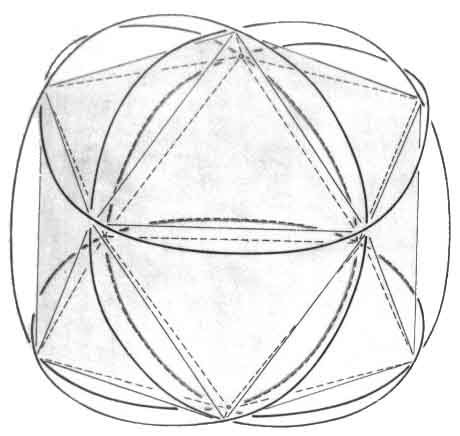
1. Table of Joos
| Elementary particle | Spin | Special characteristics |
|---|---|---|
| μ | ½ | only in charged state, „non-nucleus particle” |
| π | 0 | |
| K | 0 | |
| p | ½ | unlimited life time |
| λ | ½ | only uncharged particle known |
| Σ | ½ | |
| Θ | ½ |
2. Model table
| Teilchenmodell | Vorwärtsdrall mit Rückwärtsgang | besondere Kennzeichen |
|---|---|---|
| Tu | nein | |
| TaOu | ja | simultaneously congruent to two regular polyhedrons, only here the orbit rosette contacts the spin axis |
| Oa | ja | |
| Ha | ja | the orbit does not skip any of the polyhedron faces or edges |
| Da | ja | |
| Ia | ja | the orbit skips most of the polyhedron faces (ten out of twenty) |
| Iu | nein |
Paying close attention to both tables we can observe some relationships. If we translate the column “forward spin with reverse gear” in the second table as a “spin”, then we will find – just as in Table 1 – two small particles that do not have a “spin”. However, here we have to admit that our magnetic field theorem needs a correction that will be made below. Similarly, the column “special characteristics” in both tables contains three particles that stand out against all the other particles. These particles have the ”spin ½” in both tables; this means there is no “overlapping of characteristics”. Obviously, we are on the right track. As we have become bolder due to these indications, we will now immediately start identifying our models. Thus, we assign the model TaOu to the μ-meson because it exactly suits our concept due to its non-nucleus (shell-friendly) characteristics. According to our opinion so far, it is just a scaled-down model of all electron orbits around the nucleus. Similarly, it is not difficult to assign the model Ha to the proton because here we have a maximum degree of symmetry and full “utilization” of all polyhedron faces. Among the particles that exhibit special characteristics, only the particle
λ is left, which will be assigned model Ia.
But we know that π- and μ-meson have slightly different rest masses. At the same time, we recognize that model TaOu and model TU are very similar – their self-interaction energies and consequently their rest masses should only slightly differ from each other. By means of this conclusion by analogy we assign model Tu to the spin-free particle
π.
Thus only one spin-free particle, the K-meson, is left; it will inevitably be assigned model Iu.
The models Da and Oa are the only ones we cannot fit into our pattern of characteristics for the moment. We hope that a differentiation will be successful later when the rest masses of these particles can be calculated.
After this discussion we note with satisfaction that our conclusions by analogy are indicative of the fact that we are on track of the elementary particles because we could also have been able to find as much as 1000 models. In the same way, our “relationships of characteristics” provide a bridge between the models and the particles that still seems to be uncertain and swaying but can nevertheless lead to reasonable ideas. Of course at this point critics can argue that our procedure is not correct, e.g. we haven’t said anything so far about the uncharged particles. Thus, our collection of indications might appear as an attempt to compensate for all internal contradictions of our concept – just to introduce models that are adjusted to real conditions.
This argument would certainly be totally correct if the author wanted to introduce a theory which claims to be solidly correct in every detail. But this is not spirit and purpose of this paper. Otherwise, for example an equation or a universal principle that can be used to derive all the other special cases should be at the beginning of all considerations. This is not what we claim. First, it is generally very difficult for the reader to follow such a method. Secondly, this paper does not claim in any way completeness or precision in every respect. It shall only be a motive to examine some important points of modern quantum theory from another perspective. Moreover, the field of quantum theory has increased so enormously that it is not possible at all to cope with all of the raised problems completely. Therefore, to us this way of presentation seems to be most interesting, fascinating and, incidentally, also best understandable. Besides, we point out once more that we claimed a certain freedom of arbitrariness at the beginning of our short physical speculation. At least, we can claim so far that we have stuck to the principle of causality and therefore will continue our efforts along these lines:
Now it is time to speak about the uncharged particles and to integrate them into our model pattern, resp. To this purpose let us briefly return to our two tables of elementary particles. Here we have identified the model TAOu with the μ-meson due to its “shell friendliness”. On the other hand, it is known that there is no uncharged sister particle of the μ-meson.
Now we consider the λ-hyperon that we identify with model Ia. This particle only exists in the uncharged state.
Thus, these two elementary particles provide some kind of extreme cases with respect to the formation of charged and non-charged sister particles.
Now let us examine the spin directions of the two corresponding particle models TaOu and Ia and we must realize that also here we have two extreme cases. Whereas in model TaOu all orbital segments (read: circle arc segments) intersect the spin axis (which is not the case in any other model), in model Ia they move farther away from the spin axis than in all the other models. We will use this important indication for the construction of our uncharged elementary particles.
Now we ask a question similar to that formulated at the beginning of this paper when we explained the Pauli principle: how many additional charges fit on a spherical shell that is already occupied by a charge in the state of free self-interaction, and which rules will apply?
Initially, we justify the correctness of this question in that we may allow the existence of further charges only on the spherical shell itself. We know, in nature there is only one unit charge (with a positive or negative sign). If we allow any second charge, e.g. on any orbit found inside the given sphere, in effect we will have the case of the partly unfree self-interaction that shall not be claimed for the elementary particles. The same applies if we allow a second charge (irrespective of its sign) outside the given sphere because then we get the same situation. By means of this explanation we have demonstrated much more than expected since now we can write without more ado:
This provisional theorem is a very general formulation of the Pauli principle and applies both to all stable conditions in the shell and to the elementary particles; this will still be verified. We even strongly assume this theorem to be part of the universal extremal principle (that we are looking for) and that it is valid in general. We will call this theorem the stability theorem.
But now we want to elaborate the conditions that have to be met by further charges (apart from the charge already present there) admissible on the spherical shell:
- They must also be in the state of (approximately) free self-interaction
- The times of revolution must be identical to the time of revolution of the charge already present, otherwise these charges would – analogous to our descriptions of the homopolar bond – anytime “notice” each other and the particle decomposes. Due to these two conditions and the requirement to coexist on the same spherical shell it is certain that: the additionally admitted charges are allowed to move only along the same orbit predefined already by the existing charge.
But there can be derived even more. To this purpose, we will place two charges at any two positions on such an orbit, send them on their way and select the same sign for both. If we send them exactly in the opposite direction an impact or a mutual penetration after a short period of time (as we know too little about the charges themselves) would be unavoidable. However, in this thought experiment the stability conditions are not met; so we reject this solution as being not stable.
Next we will send the two charges on their way again, select the same sign again, but now the same direction for the two partners. After a short time they will face each other in equivalent parts of the orbit due to the Coulomb forces of external interaction; apparently we would have a minimum of temporal change of the external interaction. However, unfortunately this is not the case because we do not see any reason why these two charges should stick together at all. Thus, we reject this solution as well and formulate (what we know well already ): there is no elementary particle that is doubly- or multiply-charged.
Now we begin our speculation anew. This time we place two charges with opposite sign and opposite orientation into our orbit. This solution is apparently unstable either because it does not satisfy the stability theorem.
Finally, we inquire about the behavior of two charges with opposite sign that we send into the orbit with the same orientation. If they start such that their secant intersecting the two charges will not intersect the center of the sphere, in other words, the two charges do not always face each other diametrically, they will continuously approach each other and the stability theorem again will not be satisfied. But if we allow the two charges to be exactly opposite each other at every point of the orbit, they will start “hunting” each other without ever reaching each other. Thus, one could assume that such a model that meets the stability theorem represents a neutral elementary particle. (By the way, this model is very similar to our completely occupied spherical orbits in the electron shell .) But it can easily be seen that such a model cannot be stable at all because the two charges, as far as they only slightly deviate from the diametrical constellation, must immediately approach each other, which comes down to the case discussed above.
At this moment we can be satisfied to say that the stability theorem leads to the known solution: there are only labile neutral elementary particles. Now let us check whether this model of an uncharged elementary particle also provides information about the other characteristics of the uncharged particle that is consistent with experience. This will best be achieved if we individually examine our models of Table 2 by focusing on the theorem elaborated above. Let us start with the µ-meson (model TaOu). If here two charges with opposite sign travel diametrically along the proposed model’s orbit and in the same orientation, their joint movement will come to a sudden stop because both simultaneously complete a spin rosette, these two spin rosettes being absolutely congruent. However, the magnetic fields of external interaction prevent the free movement of the particles to be continued. The stability theorem is not fulfilled and we may say – in total harmony with the natural conditions – that there can’t be an uncharged μ-meson.
Now we come to the π-meson model (model Tu). We look along the spin axis and get the two charges started – as agreed – diametrically in the same sense of revolution. But now it becomes difficult: due to the specific character of the orbit rule outlined above there are only two constellations of the two electrons in which the electrons are actually diametrically arranged. At all other orbital points the common secant closely bypasses the center of the sphere! Thus, the stability theorem is not fulfilled in this direction. However, the deviation of the secant from the center of the sphere is oscillating, in that the particle that initially lags behind the counterpoint of the other one will lead in the next half revolution, so that one could speak about a (certainly labile) minimal change of external electrostatic interaction. In respect of the external magnetic interaction there is no reason for such a “catastrophe” as with the μ-meson,
since both charges terminate one revolution at different locations so that a synergy of the “spin magnets” is unimaginable. (Here we may speak about electrostatic and magnetic interactions because we discuss external interaction in which pure electric und pure magnetic energies exist.) Now we will take a look at Fig. 27 and ask if the magnetic fields of the self-interaction could influence each other. This question may be denied because every particle interacts with itself at every point of the orbit in another spatial direction than its partner.
We summarize: an uncharged π-meson should be extremely instable and in fact: the uncharged π-meson has the shortest decay time of all instable elementary particles.
Consequently, there must be something right in the stability theorem because it provides quite reasonable conclusions.
Now we ask: possibly we may place even more charges on the orbit of the Tu model
(π-meson)?
First we will add only one charge to the pair. This procedure must fail immediately because the already labile oscillation now becomes completely instable. But maybe we can add another “pair” to the already existing one because we have four different directions of self-interaction. Perhaps via an appropriate arrangement it will be possible for the charges not to influence each other in their self-interaction! For this purpose look at Fig. 43:
The constellation 1=e+, 2=e+, 3=e-, 4=e-
is out of question since now the charges are distributed such that the secant connecting two different charges is not even approximately constant over time. Therefore we reject this solution because it does not satisfy the stability theorem. For similar reasons we also have to reject the solution
1=e+, 2=e-, 3=e+, 4=e-
because always two identically charged electrons sometimes get in close vicinity in closely adjacent orbit segments and also remove from each other again. For these reasons we can state that an uncharged
π-meson, which decomposes into four simple charges during decay, may not exist; this is confirmed by experience.
Now, we come to the next model, the escribed octahedron. It is certain that an uncharged sister particle exists here as well, if one pair ( e+ und e- )
of charges occupies the orbit diametrically in the same sense of revolution. According to the same arguments as discussed before with the Tu model, the external interaction of the magnetic energy is equal to zero and the electrical portion of the external interaction is also an (instable) minimum.
Since we have as much as six different directions of self-interaction here, we will now check the possibility of a structure that can take up four and six charges resp. Again, four charges occupying the orbit are unstable because here the already known electrical asymmetries will apply (Fig. 44). But even for the six charges we do not find any arrangement that meets the requirement of the stability theorem. That is to say, the most symmetrical solution will be as follows:
1=e+, 2=e-, 3=e+, 4=e-, 5=e+, 6=e-.
In the figure shown we can see immediately that the lengths of the secants, which connect any electron to the oppositely charged partners, vary strongly during one revolution, so that this solution can also be rejected for the reason of instability. Consequently, there is only one neutral sister particle of the Oa type.
Now, the same examinations follow for the proton (Ha). We can repeat all the considerations that have been discussed for the model Oa since both models merge into each other due to permanent deformation and angular rotation. Thus, there is only one uncharged sister particle of the proton that contains two oppositely charged electrons. This is the neutron. Now we draw our attention to the models Da and Ia again. We treat them simultaneously because they are interrelated in the same way as the models Ha and Oa. In these two models we detect the possibility that there exists one non-charged sister particle that can take up one pair of charges. Further occupancies of this orbit seem to be rather unlikely according to the stability theorem whereas the possibility is given due to the high number of independent directions of self-interaction (a total of 10). This is interesting in that one can infer (with good will!) from the path of model Ia that here mainly the uncharged occupation but rarely the singly charged particle may be present. Unlike all the other elementary particles this model does not show an (at least closely regular) spherical-symmetrical charge distribution. Instead, the particle oscillates within a relatively narrow bandwidth around the center of the sphere. If we look at Fig. 39, we must realize that the self-interaction of this model does not continuously cover the entire path in such fixed spatial directions as, for example, in model Ha. In other words: such a strong parallelism reliably covering the entire path between the previously travelled path and the given orbit segment does not exist. Rather, with this model we have to rotate the formerly rigid spatial directions of self-interaction gradually such that kind of “revolvement” of the two paths required for self-interaction occurs. Thus, the condition of continuous coverage of the entire orbital path is met only partially.
Examining all other models with regard to this aspect we see that – apart from our proton model – none of the introduced models completely satisfies this condition (see below). Anyway, it is mostly infringed in model Ia. The charged λ-hyperon requires a “support”, which it receives with the addition of the second charge. This second charge in some way “helps” to “bridge” the range of missing self-interaction by the Coulomb attraction.
Based on this knowledge we can expand the stability theorem:
Now we come to the already announced hypothesis that none of the introduced particle models (the proton excluded) satisfies this extended stability theorem. Let us begin with model TaOu. Here, the self-interaction is not a constant value at eight points of the orbit (namely the points at which the direction of self-interaction discontinuously changes), its value of change being constant according to amount while its direction changes discontinuously.
We have already discussed the circumstances with the model Ia, where there is a “lack” of self-interaction along certain orbital segments. The same is true with the presented Model Oa. By contrast in the models Tu, Da, and Iu there is an “excess” of self-interaction along certain segments of the orbit. However, this “excess” is not directed such that the charge is fixed to the given path; instead it has a “deflecting” effect. It is only the proton (Ha), whose “excess” of self-interaction acts in the same direction and “sticks” the charge to the given orbit when the direction of self-interaction changes.
(The reader can understand these considerations easily on his own by implementing simple wire models, because it would take us too far to provide two-dimensional drawings of all figures..)
To make a long story short, for our collection of indications it will be sufficient to state that we can conclude from the stability theorem:
there is no stable elementary particle (the proton exempted).
Furthermore, we leave it to the reader to prove that the stability theorem can be used to show that, for example, two, four or even six (1 pair, 2 pairs and 3 pairs resp.) charges can be placed on the orbit of model Iu (K-meson) – also an indication that conforms to the elementary particle table provided by Joos. This means that the Pauli principle of free self-interaction does not allow only two charges on each “shell”.
The stability theorem, however, is a real goldmine. If it is considered to be universally valid, it still contains much more: one can understand the direction quantization in the Stern-Gerlach experiment without any problem. We will now use it to demonstrate that in an exterior field our two particles (π-meson and K-meson) without “forward spin with reverse gear” will show a behavior principally different from all the other model particles . In these models it can be seen at one glance that all the directions of self-interaction are grouped as a bundle closely around the “spin axis” standing perpendicular to the plane of projection in Fig. 26 and Fig. 41. Our two particles would be badly advised to turn said axis toward the external field when encountering external fields because every other spatial direction perpendicular to this axis causes the directions of self-interaction to diverge considerably more from the direction of the external field. Namely, for all of these directions the magnetic field, that the particle can generate according to the magnetic field theorem, is equal to zero. Therefore, the case in which the “spin axis” is oriented in the direction of the external field may virtually not occur as an unstable condition. We see that both particles do not show the Stern-Gerlach effect and, thus, they must have the spin of zero. On the contrary, for all the other particles the setting of the spin axis along the direction of the external field is the most stable one.
Now we come to the rest masses of our particle models. Initially we will restrict ourselves to the singly-charged particles. More indications can be obtained from a more detailed study if one poses the question: what actually is the rest mass of a particle?
At the moment we have to bear in mind our statement that the rest mass is equal to the self-interaction energy divided by the square of the speed of light. Further, it is useful to consider the equations that describe the pair generation of, for example, an electron and a positron:
| E = m0c² | rest energy of a charge |
| E = h ⋅ ν | minimum energy of a ∂-quant (required for the pair generation) |
From this follows by equating:
| m0c² = h ⋅ ν = h * | c |
| λ |
Benutzen wir nun die Gleichung: h = e0²c ⋅ const, so gilt:
LI
m0 = const ⋅ e0² λ
Thereby, we obtain the very important indication that the rest mass can depend only on one single variable that has the dimension of a length. This is a result that makes every attentive reader think about the smallest length introduced by Heisenberg;we will try to find an illustrative explanation for this. For this purpose, let us have a closer look at a charge. The property of a charge is to be the well (or sink) of a space. As it is obviously a real, existing object that can have an effect on itself or on other charges, its dimension may not be equal to zero (i.e. the mathematical point). Otherwise it would not exist. If, however, it has finite dimensions, there must be a smallest radius of a circular orbit on the circumference of which this charge is barely able to interact with itself. This smallest curvature radius could be identical to the shortest length. But since the free self-interaction must certainly follow certain rules, there should also be a revolution period for this smallest curvature radius. This revolution period shall be the smallest time introduced by Heisenberg.
We obtain another indication recognizing that a regular polyhedron is completely determined when a single edge length is provided. We already know that a charge sticks to the orbits of self-interaction by its own magnetic fields. Therefore, we can write:
Hence:
And in fact: even at this point clarity does not disappear, since it would be highly illustrative if self-induction coefficients, providing a perfect example for the inertia of a current flow, could be assigned to the rest masses (the site of the inert masses).
Should the analogy between inert mass on the one hand and self-induction of an electric circuit on the other hand, described in every textbook of physics for a better understanding of self-induction, be eventually reality rather than mere analogy? Such an interpretation is so irresistible and harmonious that one is determined to collect even more arguments in favour of this theory; however, one should be careful in doing so, because the enthusiasm for such a plan could blurr the picture. Anyway, such an opinion could really be the key to understand Einstein‘s mass energy relationship E = m0c². To demonstrate this we write three equations one after the other and discuss their interrelations:
| E = m0c² | Einstein’s mass energy relationship | ||||
|
Potential energy of a current-carrying conductor (energy of self-induction) |
||||
|
equation LI (rearranged) |
Now, we rearrange the second equation for one electron as usual:
|
|
Now for the second equation we can write:
LII
E = 1 L11 e0² * V² 2 s²
Further:
E = const * e0² c² λ
If we consider this equation and the adjoining equation, we will find an exceptionally close relationship. In each of the equations one can find on the right-hand side the square of the elementary charge, multiplied by a magnitude of the dimension cm-l and the square of a speed. Apparently we are on a path which seems to make sense of the two theorems specified above.
Indeed, we have got an interesting result from the requirement that rest mass and self-induction coefficient be directly proportional:
It is well-known that the self-induction coefficient is entirely independent of the electrical current and only depends on the geometry of the current flow. Consequently, the rest masses of proton and neutron, for example, should be more or less identical (if we disregard the slight orbit deformation caused by the Coulomb forces)!
More is not admissible at this point, although, e.g. equating the two equations and, thus, further speculations appear to be tempting. This is forbidden because the left “classical equation” contains L11 that has not yet been characterized. If we use the standard formula to calculate the self-induction of one single charge travelling along any space curve, we will fail in the same way as with the use of the Biot-Savart law, because this formula has been derived from the perspective of external interaction. Thus, we have to try to rewrite this equation again for one single charge, while considering the knowledge obtained above, particularly that of the magnetic field theorem.
But first, let us take down a formula to calculate an induction coefficient of the external interaction between two circuit loops:
Again we discover an exeptionally valuable indication: namely, it is “common” that the integration directions of the two integrals are selected such that L12 becomes positive. Now we expect the formula of the self-induction coefficient of a single charge on an orbit of self-interaction to be a similar double integral. However, from our perspective we still do not see any argument for necessarily integrating such that L11 becomes positive! But as we already see from far the self-induction coefficient to be related to a mass, at this point we may introduce a negative mass, namely antimatter!
At this point at the latest every reader will recognize that our way branches out more and more into different directions. We have not even started to calculate the rest mass, but we are already speaking about antimatter. Yes, now the flood of ramifications to follow is so manifold that we could get off track almost unnoticeably. Moreover, the calculations to be made may easily overwhelm a single person; particularly if one takes into account the point of view from which these considerations have developed. The reader will understand this comment at once if he takes into account the reference literature listed at the end of this paper.
To make a long story short, it would be high time to lay aside the pen if by means of numerous ramifications it can be shown that the selected way leads to fertile ground, because then the objective of this paper would have been achieved. So let us save ourselves a great many of proofs and leave it to a more competent body – just because we do not want to commit still more false steps due to the pure lack of knowledge . While blocked for the professional theoretician, such a retreat is advisable to the amateur at an appropriate point of time!
The present paper attempts to penetrate into the world of quantum theory by using the causality principle and to pave a way for the elimination of some basic problems related to quantum theory for those who are ready to revise their traditional point of view. There is only a smallnumber of proofs in favour of this new standpoint, whereas the number of indications is so overwhelming that it is justified to say: sometimes it may be absolutely fascinating to take such a point of view. For example, it can be shown easily that the new standpoint is definitely consistent with the postulates of the special relativity theory. What is more, it provides a deeper understanding of the general relativity theory that starts out from the equivalence of inert and heavy masses. The definition of mass suggested in this paper directly leads to the theorem used by Einstein as a postulate of the aforementioned equivalence if the heavy mass of a body is understood as a diffuse “magnetic field” generated by multiple self-interactions. Furthermore, according to the author’s opinion, there exist only the following physically relevant structures: wells und sinks of the space as well as the appropriate fields. Said fields probably should behave more or less in the following way: all dynamic processes (temporally changing) correspond to a maximum of the temporal change of external and self-interaction, while all stable processes (constant in time) correspond to a minimum of the temporal change of external and self-interaction. Thereby it should be possible to describe all processes within a measuring system which only requires three universal constants:
- speed of light
- elementary charge
- shortest length (or time)
Presumably the gravity constant will be derived from the third universal constant one day. At the same time, within the scope of such a theory the existence of gravitational waves is out of question as well. However, the venture of calculating the metrics of the space according to the mass distributions is by no means hopeless.
In the same way, it can be expected that it is also possible to put in order the table of elementary particles. Such a theory, once established, can be expected to provide a complete picture of the atomic nuclei, for then it will become easy to compose the nuclei from orbited hexahedrons and to identify and calculate their “exchange forces” in terms of coupled self-interaction energies. Further, such a theory will certainly describe the mass defects in terms of changes of self-interaction energies via coupling. Thus we see, that the big mystery of “nuclear forces” can definitely be solved in the foreseeable future. Also, this theory will be able to explain the short range of the nuclear forces. After all, it can be expected that such a theory can also throw some light on the discussion of the “shell or droplet model”.
Likewise, the radioactivity should be expected to reach the state of calculability if one assumes that the protons and neutrons forming the nucleus do not necessarily result in configurations corresponding to the stability theorem.
Furthermore, one day it will possibly be shown that the state function
Ψ used in quantum theory can be derived from the theory of elliptical functions because solving the elliptic integrals normally requires such a lot of effort that the formerly productive mathematical procedures will continue to be used, though no longer as a dominant element but as an auxiliary means to explain nature.
Lastly, such a theory could provide a new outlook on “mysterious” natural phenomena such as superconduction, superfluid, very hard cosmic radiation or ball lightning, provided the new standpoint is sufficiently substantiated.
But perhaps it will be possible to deduce even more from such a theory in future: after all, the on-going increase of entropy in nature is one of the most important results of the classical theory. The world of elementary particles, however, appears to be a world of ultimate order and harmony, a world of self-interaction (rather than a diffuse image of a “random”, “probable” and impenetrable thicket). This world does not know any kind of disorder and therefore all the systems that are predominantly composed of systems of self-interaction must feature a continuously decreasing entropy. This could be the theory of Darwin (the origin of life and the development of all biological systems from low to high). Accordingly, nature is not only causal but presumably also symmetric; maybe there is such an organizing principle being effective even in the vast expanse of the universe controlling the formation of fixed stars? At this point we do not dare to make presumptions but nevertheless it should be asked if perhaps such an organizing principle balances out the predicted “heat death”?
One thing, however, is extremely depressing: we have not even been able to roughly answer our initial question and still face the big mystery: what actually is a photon, how is it formed and how does it cease to be?
But it is just this question which brought us such a lot of small pleasures along our journey of exploration that we should not leave without seriously trying to answer it to some extent. Thus we continue our efforts once more:
These efforts finally culminate in an aforementioned extension of the magnetic field theorem. Therefore, we will now have a look at the figure shown above: a negative charge follows a space curve that satisfies the magnetic field theorem in the direction of the arrow (Fig. 45). Then the north pole of the magnetic field is found in the direction of the arrow according to the “right-hand rule”. Now, let a positive charge travel in the same direction (Fig. 46). The north pole then must be be in the opposite direction. We see that the “left-hand rule” has been designed for the positive charge. Consequently, positive charges generate space eddies that are assigned to a left-hand coordinate system, whereas negative charges generate space eddies that are assigned to a right-hand coordinate system.
This is still nothing new, but now it becomes interesting: shortly after the calculation of Planck’s constant, we had given an illustrative explanation of the self-interaction mechanism and failed to examine the direction that is perpendicular to the plane of the eddy. But it is clear to the observer that the flux lines can be pushed aside to the convex part of the orbit in only one direction – i.e. in the forward-movement direction of the charge. Thus, the magnetic space eddy appears, depending on the sign of the generating charge, as a right- and left-hand helix, respectively. Now we look at our proton model in the spin direction (Fig. 47). We have to acknowledge that the individual rosette lobes will travel in a direction such that the charge alternately follows a right- or a left-hand helixbolt. Should it even be possible that an external electron, used as a probe, be so “half-blind” that it only perceives the movement of the positron that fits to the (own) right-hand system? Maybe this could be the extension of the magnetic field theorem we are looking for?
Such a sentence would be simple to illustrate,because if two magnetic fields with right- and left-hand systems collide, it would be like a nut with a right-hand thread that has to be screwed onto a bolt with a left-hand thread.
For a charge in the state of self-interaction, this condition is met for every part of the orbit. However everything changes if we discuss external interaction, because now it is important to which coordination system the “generating” and the “measuring” charge belong. But because all measurements in particle physics must be attributed to the movement of the electrons (because they are available for measuring) or be compared to their movement considered a measurement standard, one could be right to assume that only half the expected interaction will occur in a model belonging partly to the right-hand and partly to the left-hand system. Maybe this is the real meaning of the term spin?
Of course we toy with such an idea because we already know that the “calculation” of the gyromagnetic ratio of the electron must be wrong (due to its present rest mass) and we only consider it as a fortunate coincidence that the plausibility considerations lead to the correct result
But again there appears one of those ramifications (e.g. the calculation of the magnetic moment of proton and neutron) and therefore we will break off here and return to the light quantum. It represents a particle with a zero rest mass. Now we have to select one out of two options that will be explained in detail below.
First option: a particle with a zero rest mass cannot exist according to our previous formulations because all closed continuous kink-free orbits on spherical surfaces or ellipsoidal surfaces meeting our 5 requirements must “return” sometime. Thus it will always be possible to find at least one direction in space in which an external observer can notice a right-hand and left-hand spin and therefore be able to detect a mass (read: potential, magnetic energy, as seen from outside). But everything would be wrong, because for the calculation of our quantum of action we have assumed light quanta to be always a product of their self-interaction – an idea that we do not like to accept.
Second option: our requirement that self-interaction should only be possible on spherical or ellipsoidal surfaces is too rigid and has to be extended. In fact, it has arisen from the demand for constancy of the absolute value of the angular momentum, and it seems that this demand is of general nature.
It is not a contradiction to the requirement of constancy of the absolute value of the angular momentum (using once again the “classical” idea by way of exception) if we introduce a space curve for the photon field that is positioned on a cylindrical surface bent into a ring (See Fig. 48).
Now, in “spin direction” we see a toroid that is known for its extremely good shielding of the magnetic field to the outside. This provides an option to introduce a particle with a zero rest mass. What is even more: it is just this particle that may illustrate the existence of antimatter because a toroid can be wound clockwise and counter-clockwise. Might it be that th “ominous” neutrino is the photon of antimatter? Should this particle correspond to the field lines of a counter-clockwise toroid? Maybe the free electro-magnetic fields are able to perform self-induction? Maybe these fields can be compared to an ideal liquid in which free space eddies can develop and cease to exist (exactly because the Helmholtz’ eddy theorem only applies to conservative forces in such a liquid, for conservative forces are no longer imaginable with self-interaction). Questions upon questions which the author is unable to cope with and that are addressed to all readers!
bibliography:
- Joos, G. „Lehrbuch der theoretischen Physik” 10. Auflage, Akademische Verlagsgesellschaft, Geest & Portig K.-G., Leipzig 1959
- Grimsehl, „Lehrbuch der Physik” Bd. I bis IV B.G., Teubner Verlagsgesellschaft, Leipzig 1964
- Gehrtsen, Ch., „Physik, ein Lehrbuch zum Gebrauch neben Vorlesungen” Springer-Verlag, Berlin, Göttingen, Heidelberg 1958
- Heber - Weber, „Grundlagen der modernen Quantentheorie” Teil 1, B.G. Teubner Verlagsgesellschaft, Leipzig 1964
- Westphal, W.H. „Physik - ein Lehrbuch” 20. u. 21. Auflage, Springer-Verlag, Berlin, Göttingen, Heidelberg 1959
- Bronstein/Semendjajew, „Taschenbuch der Mathematik” B.G. Teubner Verlagsgesellschaft, Leipzig 1962